Mann-Whitney U and Wilcoxon Signed-Rank Test
The Mann-Whitney U test compares two groups on a numeric response without assuming normality, working on ranks instead of raw values; the Wilcoxon Signed-Rank test does the same for paired measurements. This tutorial explains the W and V statistics, how to choose between the two tests, what the Hodges-Lehmann interval tells you, and how to run the whole analysis code-free… Read more …
The Mann-Whitney U test is the nonparametric, rank-based alternative to an independent-samples t-test for comparing two independent groups on a numeric response, used when the data are ordinal, the sample is small, the distributions are skewed, or normality simply cannot be assumed. Its paired counterpart, the Wilcoxon Signed-Rank test, is used when the same experimental units are measured twice. Because both work directly on ranks rather than raw values, neither needs a data transformation.
This tutorial introduces the basic concepts behind rank-based two-sample testing, including how the W and V statistics are formed, how to decide which of the two tests your design calls for, and what the Hodges-Lehmann confidence interval adds to a bare p-value. It then provides a step-by-step guide to performing the analysis in the RAISINS platform: preparing your data, choosing the test type, reading every part of the results table, reviewing the six available plots, and using the built-in RA-One AI assistant to make sense of the output. No programming knowledge is required.
1 What is the Mann-Whitney U Test?
The Mann-Whitney U test asks whether a numeric response tends to take larger values in one of two independent groups than in the other. It is the rank-based counterpart of the independent-samples t-test, and it is the test to reach for when the t-test’s assumptions are uncomfortable: small samples, visibly skewed distributions, obvious outliers, or ordinal responses such as a 1-5 sensory score, where the distance between “3” and “4” is not guaranteed to mean the same thing as the distance between “4” and “5”.
The mechanism is simple. All observations from both groups are pooled and ranked from smallest to largest, ignoring which group they came from. If the two groups genuinely differ, one group’s observations will cluster among the low ranks and the other’s among the high ranks. The test summarises that separation in a single statistic, W, and converts it to a p-value. Because only the ordering of the values is used, the result is unaffected by how the raw numbers are scaled, and no transformation is required.
A significant Mann-Whitney U test tells you the two groups differ in location, that one tends to produce larger values than the other. It does not, on its own, tell you by how much. That is what the accompanying confidence interval is for (Section 8).
The Mann-Whitney U test and the Wilcoxon rank-sum test are the same test, discovered independently and published two years apart. You will see both names in the literature, and some software reports one where others report the other. RAISINS reports the statistic as W, following R’s own convention.
This is not the same as the Wilcoxon Signed-Rank test, which is the paired test described in Section 2. The similar names are a well-known source of confusion.
2 Mann-Whitney U or Wilcoxon Signed-Rank?
This module performs both tests, and the choice between them is decided entirely by your experimental design, not by the data. The Select Test type control at the top of the sidebar is where you make it.
Use the Mann-Whitney U Test when the two groups contain different experimental units: a treated plot and a control plot, two varieties, two locations. The groups need not be the same size, and there is no correspondence between the first observation in one group and the first in the other.
Use the Wilcoxon Signed-Rank Test when the same unit is measured twice: before and after a treatment, two leaves from the same plant, the same panellist scoring two samples. Here the observations come in matched pairs, and the test works on the differences within each pair rather than on the two groups separately. The statistic is reported as V rather than W.
Choosing the wrong one is a real analytical error, not a formatting preference. Treating paired measurements as independent throws away the pairing that makes the design sensitive, and usually costs you the ability to detect a real effect. Treating independent groups as paired is worse: it manufactures pairings that do not exist, and the resulting p-value is not interpretable.
If you are unsure, the module has a built-in explainer. Click “When should I use Mann-Whitney U test vs Wilcoxon Signed-Rank test?” just below the Test type control.
3 Getting to the Module
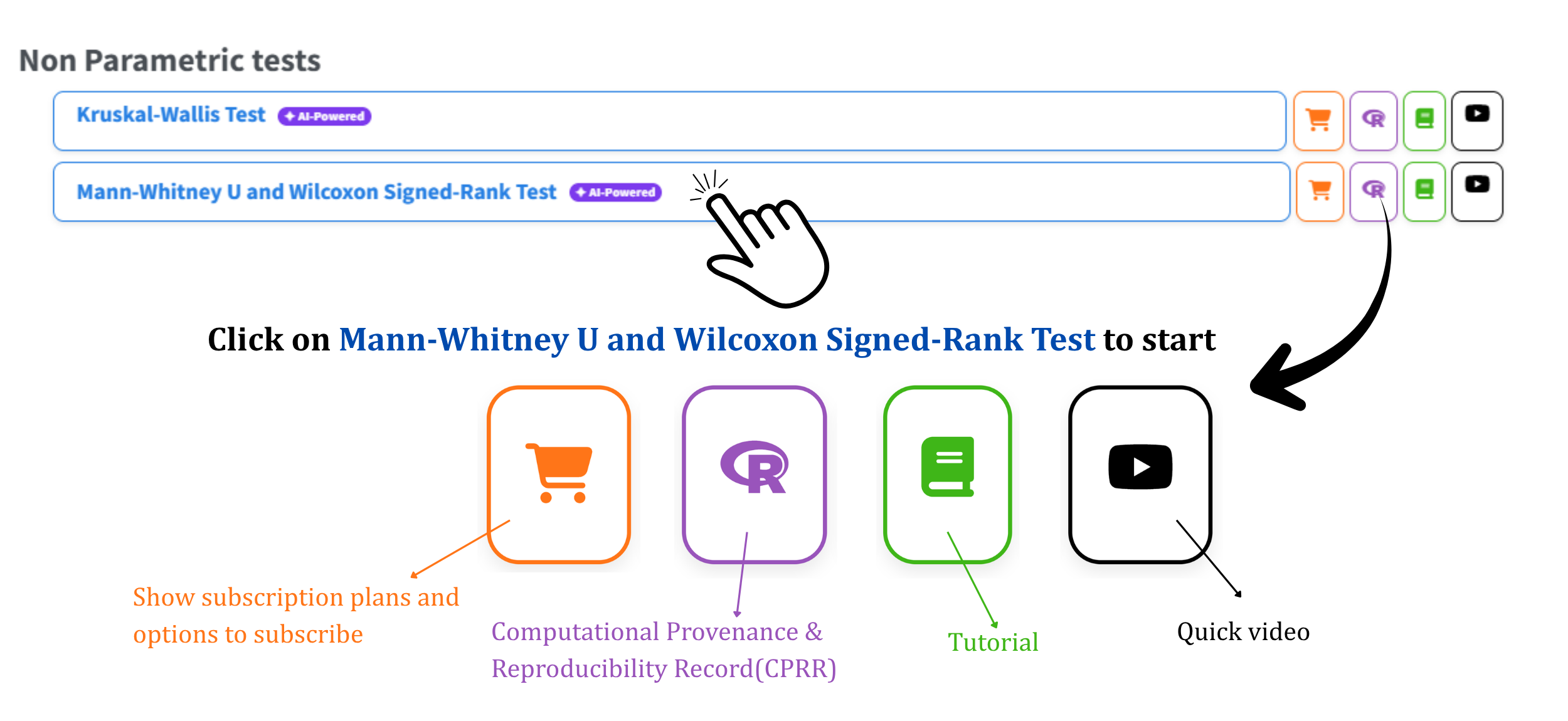
Open the RAISINS home page at www.raisins.live and go to the Non-Parametric test section. Select the Mann-Whitney U and Wilcoxon Signed-Rank Test module (Figure 1).
No programming knowledge is required. You upload your data, choose the test type, select the group column and one or more response variables, and RAISINS performs the complete analysis and produces publication-ready output.
3.1 Computational Provenance & Reproducibility Record
CPRR (Computational Provenance & Reproducibility Record) provides a transparent and comprehensive record. Click on the icon shown in Figure 1 to access CPRR and know about the computational workflow performed during the analysis. The record for this module states the R version and the exact version of every package used, names the specific function behind each reported result. CPRR lists every default parameter and decision rule applied by the module and provides fully runnable R code that reproduces each analytical step. Users can execute the code in R to independently reproduce and verify the results. It carries its own DOI.
To cite the platform itself in a paper, thesis, or report, use the RAISINS citation, available in APA, Harvard, and BibTeX formats at www.raisins.live/citation.html. That is the primary reference, and for most manuscripts it is all you need.
The CPRR for the Mann-Whitney U and Wilcoxon Signed-Rank Test module is at www.raisins.live/module_record/mwu.html.
Cite the RAISINS paper as your primary reference for the platform. Add the CPRR as supporting documentation when a journal asks for details of the computing environment, or when you want your methods section to be precise about versions and functions rather than saying “analysis was carried out using an online tool.” The CPRR supports the citation and ensures computational reproducibility.
4 Preview Mode and Quick Tour
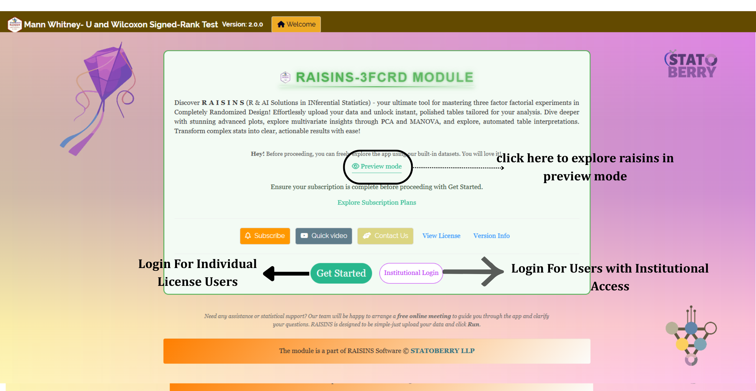
You can explore the entire module before subscribing by using Preview mode on the Welcome page. It loads the built-in demo datasets, so you can try every feature, including both test types and all six plots, without uploading your own data.
On first login, you are also offered a choice between Take the tour and Skip. Taking the tour launches an interactive, guided walkthrough that highlights each navbar tab and sidebar control in turn and explains what it does, from uploading a file all the way through to downloading a report. You can replay it at any time from the Quick Tour tab in the top navigation, whether or not you took it the first time.
5 The Example Dataset
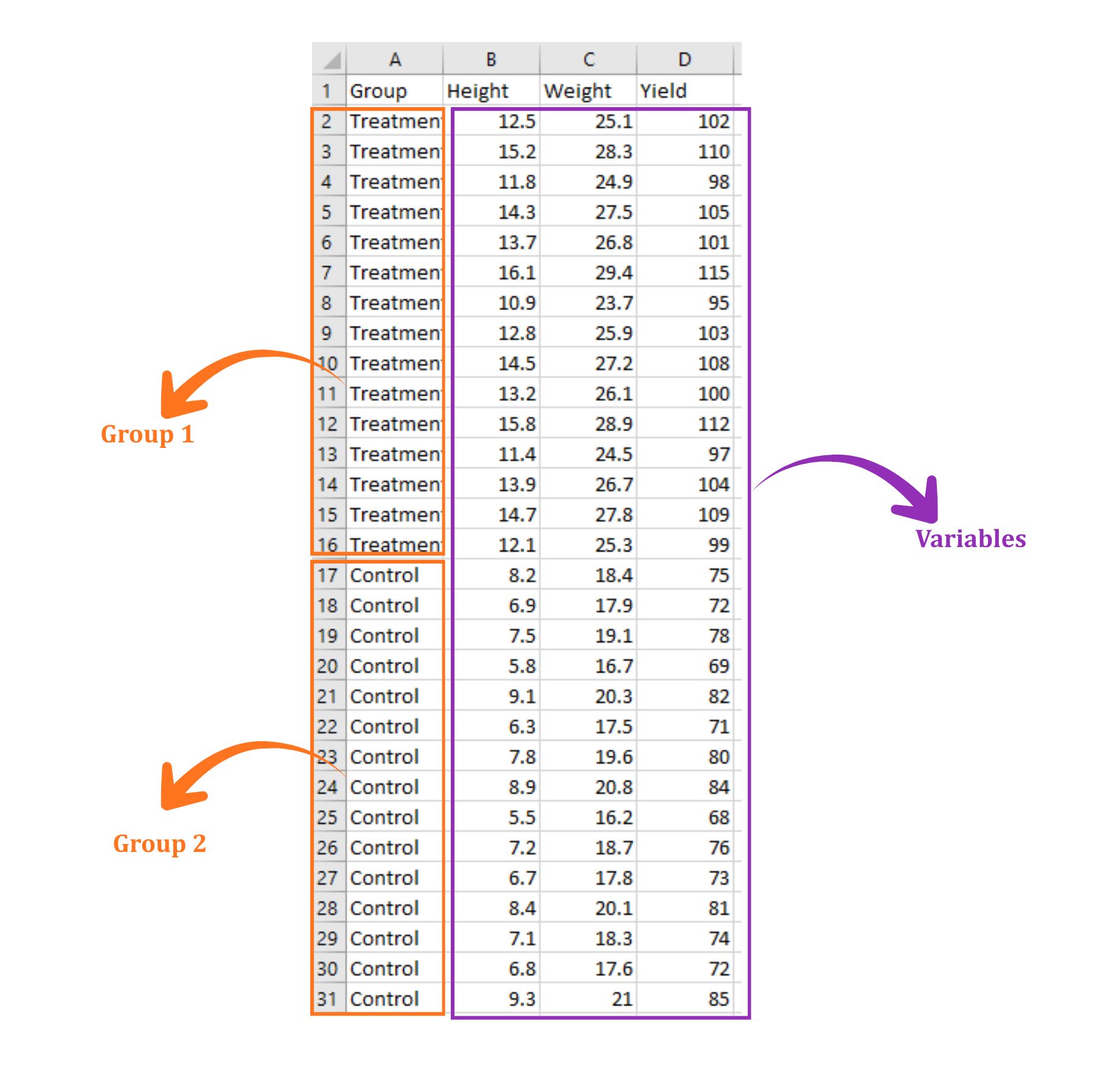
The worked example used throughout this tutorial is the module’s own bundled demo file, dataset1.csv. It records a simple two-group comparison: 15 experimental units under a Control condition and 15 under a Treatment condition, each measured on three response variables, Height, Weight and Yield (Figure 3).
The layout is the one the module expects, and it is worth reading carefully before preparing your own file. There is a single Group column holding the two group labels, and one further column for each response variable. Every row is one observation.
6 Preparing Your Data
RAISINS accepts .csv, .xls and .xlsx files. CSV is recommended: it is lighter, faster to process, and less prone to hidden formatting. The How to save my file as CSV? entry in the FAQs tab walks through the export step in Excel with screenshots.
Your file needs to satisfy a small number of rules:
- One worksheet only, with no notes, totals, or annotations outside the data block.
- Row 1 holds the column names. Start in cell A1, with no blank rows above.
- One Group column containing exactly two distinct labels. More than two, and the module will stop and tell you so; a two-group test cannot be run on three groups.
- One column per response variable, containing numbers only.
- Column names should start with a letter and contain only letters, numbers, dots or underscores. Avoid spaces, units and special characters, they resurface as awkward axis labels in the plots.
If you would rather not build the file by hand, there are three alternatives inside the app.
6.1 Create the dataset inside RAISINS
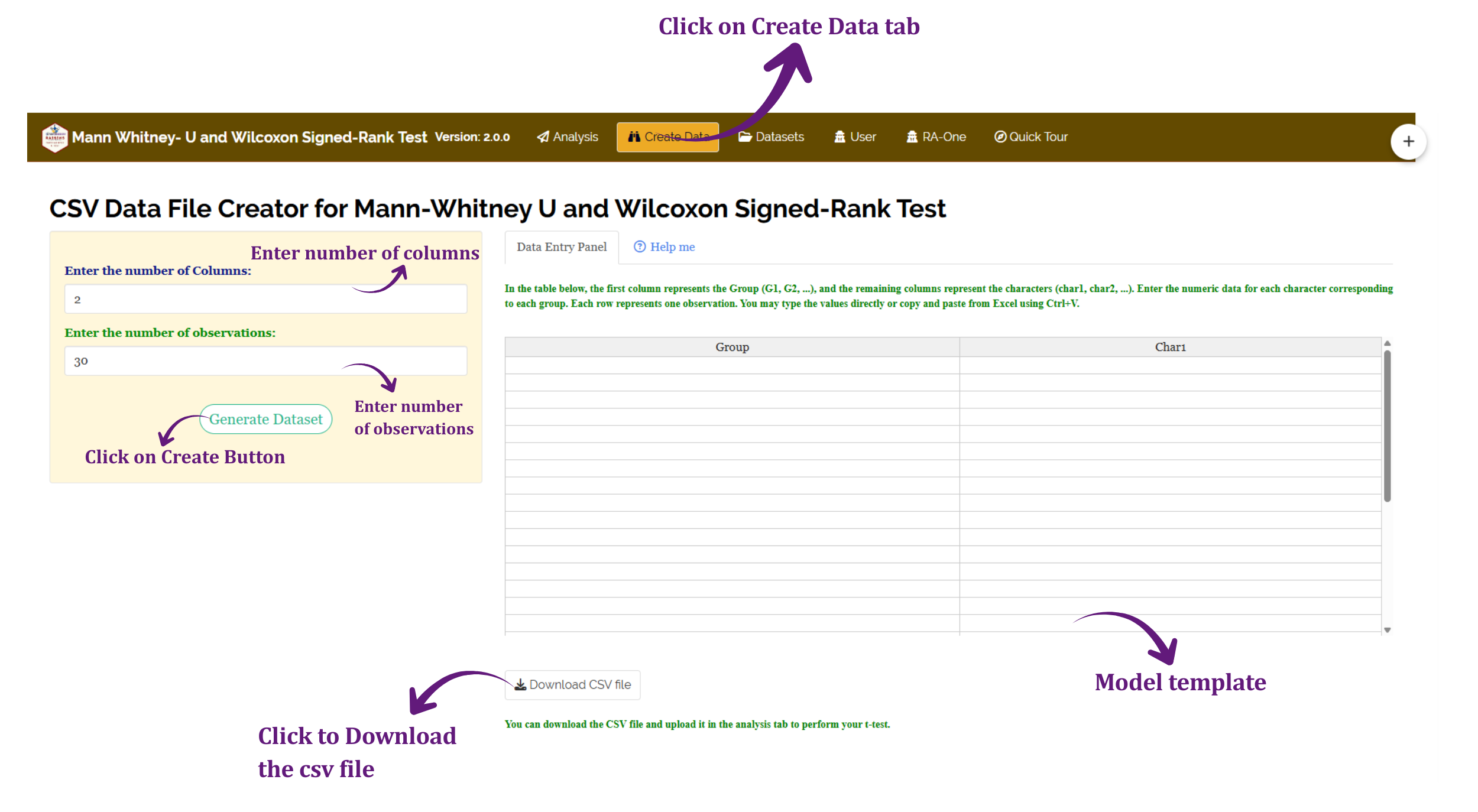
The Create Data tab builds a ready-made template. Enter how many observations there are in each of the two groups and how many Characters you measured, then click Generate Dataset. The table appears with the Group column already filled in - all the rows of Group A first, then all the rows of Group B - so you only need to enter the response values, either typing them directly or pasting from a spreadsheet. Rename Group A and Group B to your own labels by typing over them. The finished table downloads as a CSV, ready to upload.
The two groups may be different sizes for the Mann-Whitney U test; for the paired Wilcoxon signed-rank test give them the same size, since rows are paired in order (Section 2).
6.2 Start from a model dataset
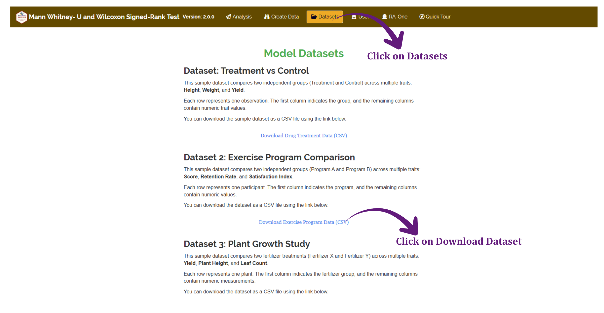
The Datasets tab holds the bundled model files. Download one, replace its contents with your own measurements while keeping the structure intact, and upload it back. This is the quickest route if you are unsure about the expected layout.
6.3 Ask RA-One to build it
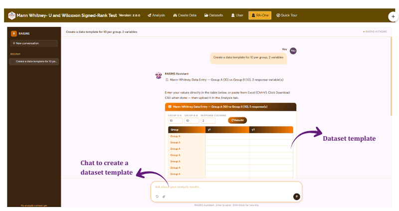
The RA-One assistant can generate a correctly structured two-group template directly in the chat. Describe what you need, for example “create a data template for 10 per group, 2 variables”, and it produces an editable table you can fill in and download as CSV.
7 The Analysis Tab
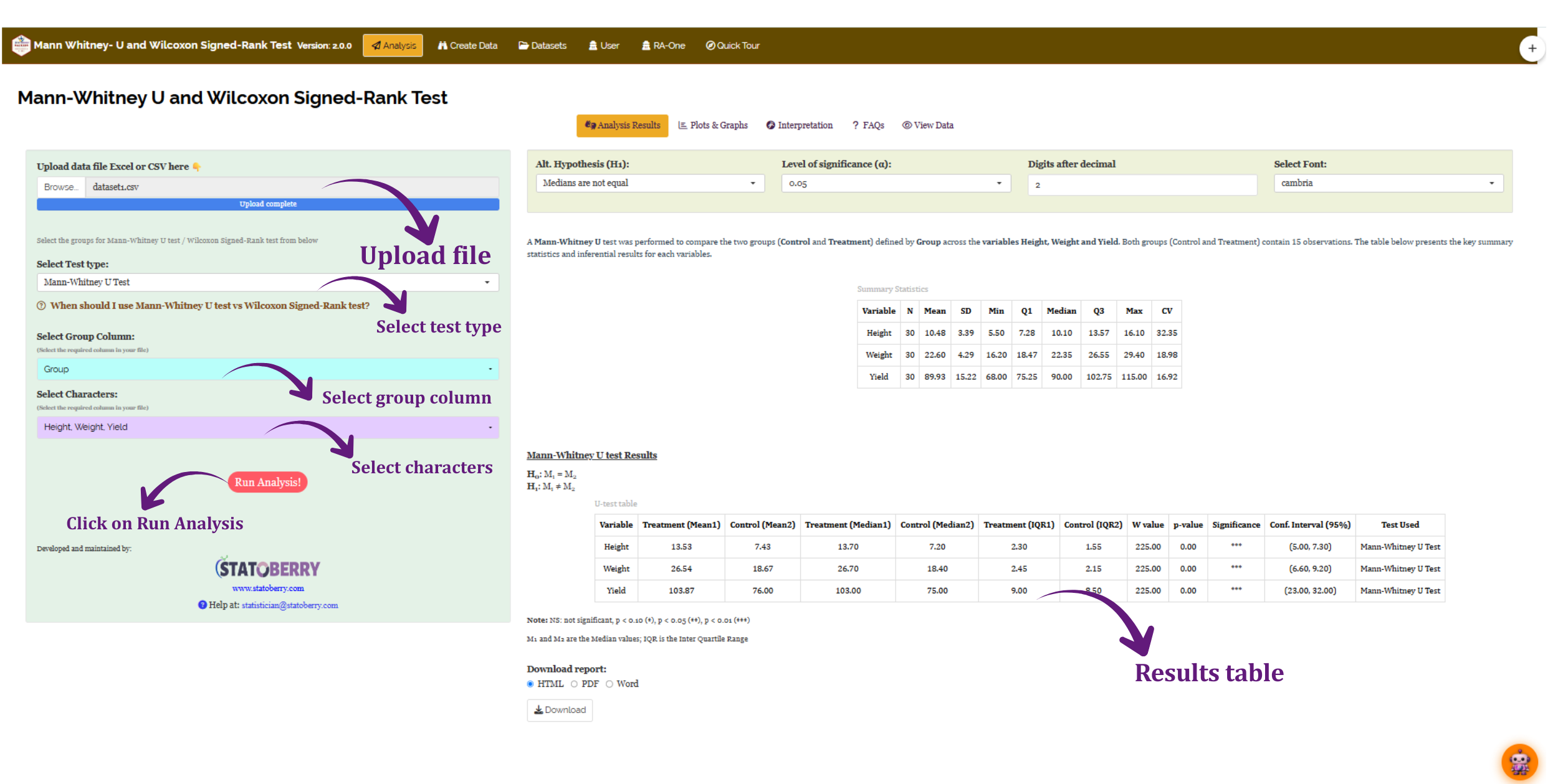
The Analysis tab is the main workspace. Upload your file with the Browse control at the top of the sidebar; RAISINS confirms the upload and reports how many rows and columns it found.
The sidebar then presents the analysis controls in the order you need them (Figure 7):
- Select Test type - Mann-Whitney U for independent groups, Wilcoxon Signed-Rank for paired measurements (Section 2).
- Select Group Column - the column holding your two group labels.
- Select Characters - the response variable or variables to analyse. You may select several; each is tested independently and gets its own row in the results table.
Above the results, a control panel sets the alternative hypothesis, the level of significance, the number of decimal places, and the font used in the output.
The default, “Medians are not equal”, is the two-sided test and is the right choice unless you have a directional hypothesis fixed before seeing the data. The one-sided options, “Median 1 is less than Median 2” and “Median 1 is greater than Median 2”, are more powerful in the direction they test, but they cannot detect a difference in the other direction at all. Choosing a direction after looking at the results inflates the false-positive rate and is not defensible in a manuscript.
When everything is set, click Run Analysis!.
8 Analysis Results
The results table carries one row per response variable, so a three-variable dataset produces three rows in a single table (Figure 8). Reading across a row:
- Mean 1 / Mean 2 and Median 1 / Median 2 - the average and the middle value in each group. For a rank-based test the median is the more relevant summary; the mean is provided for context, and a large gap between the two is itself a signal that the distribution is skewed.
- IQR 1 / IQR 2 - the interquartile range in each group, describing spread without being distorted by outliers.
- W value (or V value for the paired test) - the test statistic.
- p-value and Significance - the probability of seeing a separation this extreme if the two groups really had the same distribution, with stars marking the conventional thresholds.
- Conf. Interval - the confidence interval for the difference in location between the two groups.
- Test Used - the test actually applied, recorded explicitly so the table remains self-documenting when exported.
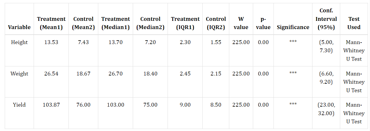
The p-value answers “is there a difference?”; the confidence interval answers “how big, and how precisely do we know?”. RAISINS reports the Hodges-Lehmann estimate of the location shift and its distribution-free interval, in the original units of your response variable.
An interval that excludes zero corresponds to a significant result at the same α. But a narrow interval close to zero and a wide interval spanning most of the plausible range are very different findings, even though both may be reported as “not significant”. Journals increasingly expect the interval alongside the p-value; quoting both is stronger than quoting either alone.
The significance stars follow the module’s own thresholds: *** for p < 0.01, ** for p < 0.05, * for p < 0.10, and NS otherwise. Note that a single star marks the 0.10 level, which is weaker evidence than the 0.05 convention many readers assume. State the actual p-value in your write-up rather than relying on the stars alone.
9 Plots and Graphs
The Plots & Graphs tab contains the complete set of visualisations. Select a plot using the row of icon buttons at the top of the tab. The selected plot appears below, with a Settings dropdown in the corner for customization.
Every plot can be customized. You can change the title, the axis labels, the colours, the point size and transparency, and the theme. Every plot can also be downloaded in PNG, JPEG, TIFF, PDF or SVG format, at a resolution you choose.
The default settings are publication-ready, so the figures are clear without any adjustment.
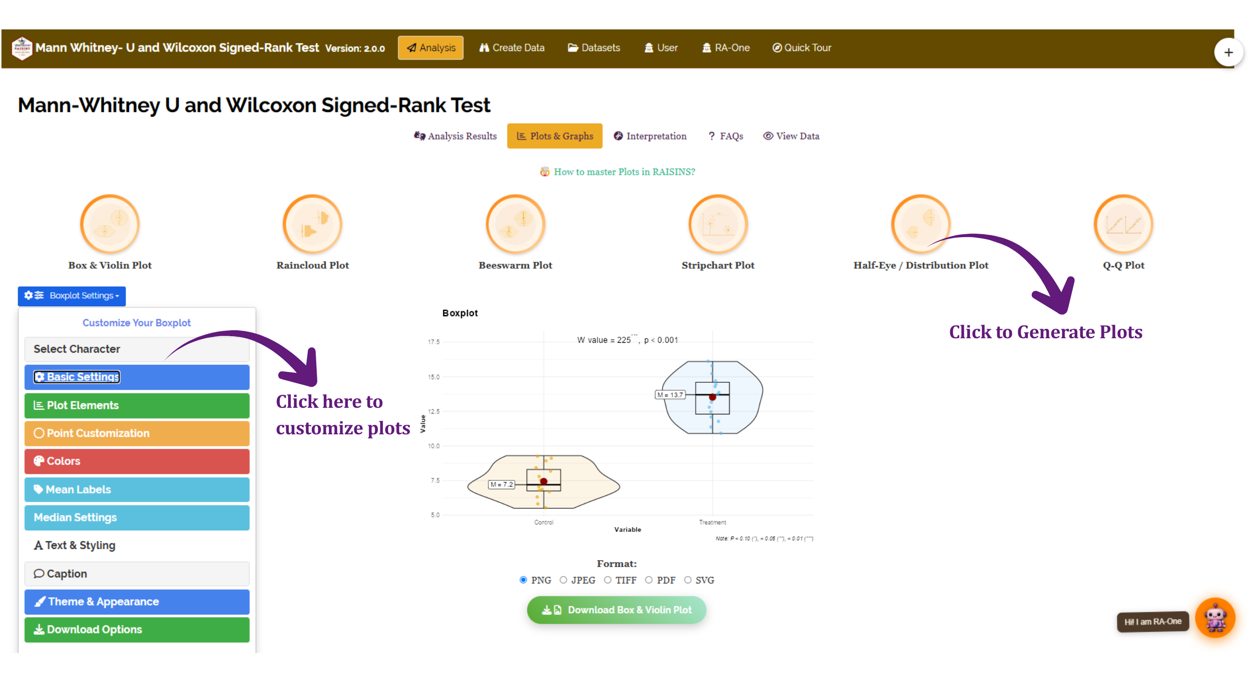
All six plots show the same two-group comparison, but each answers a slightly different question. The first four display the observations themselves; the last two describe the shape of each group’s distribution.
Hover over any thumbnail below to see what it displays.
For a two-group comparison the raincloud plot is usually the most informative single figure, because it shows the distribution, the summary statistics and the raw observations at once. With small samples, prefer a plot that shows every point (beeswarm or stripchart) over one that only summarises them, so the reader can judge the spread for themselves.
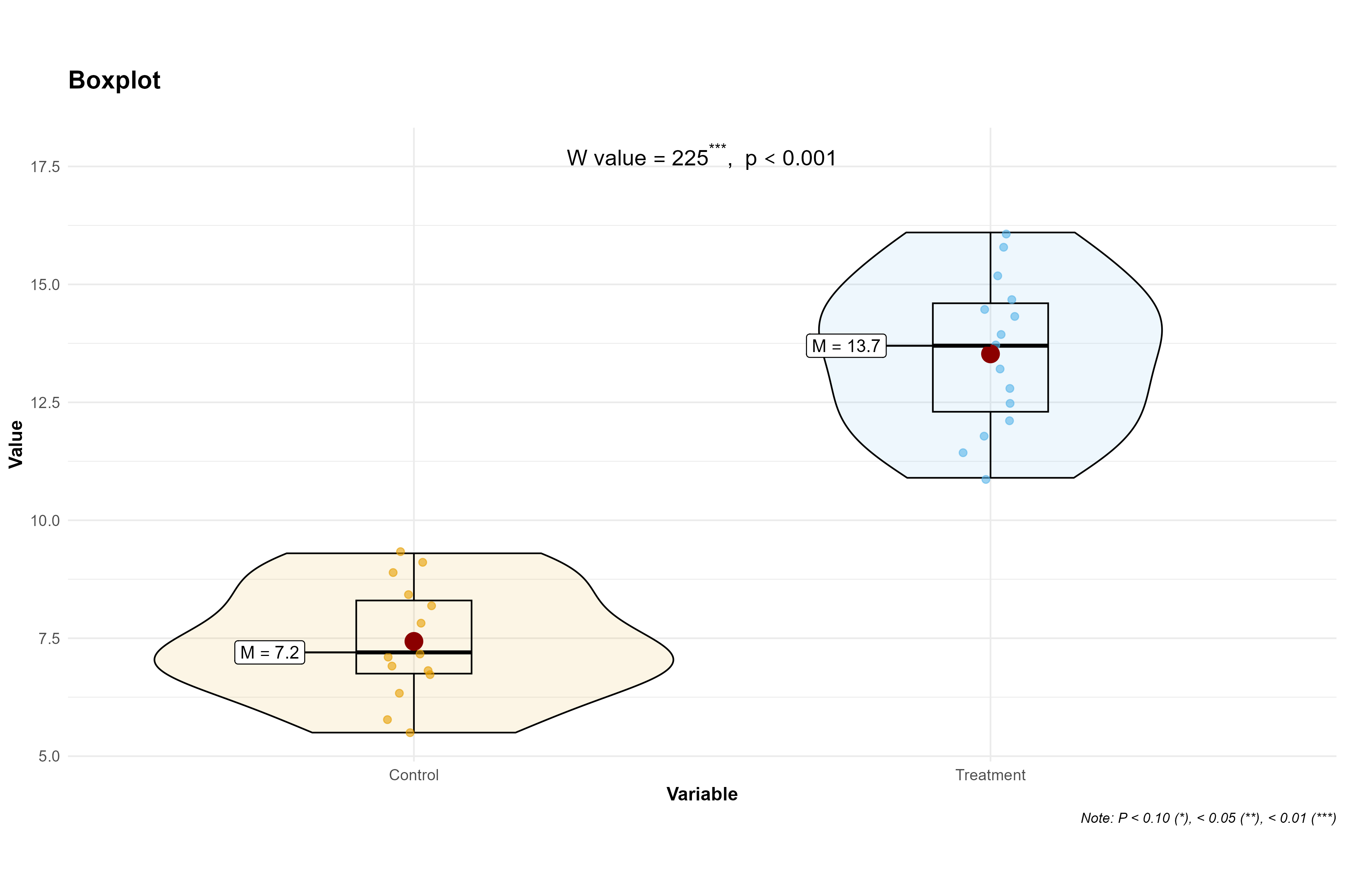
Box & Violin plot. The box gives the median and quartiles, the whiskers the range, and the violin outline the shape of the distribution. The standard choice for a two-group comparison in a manuscript.
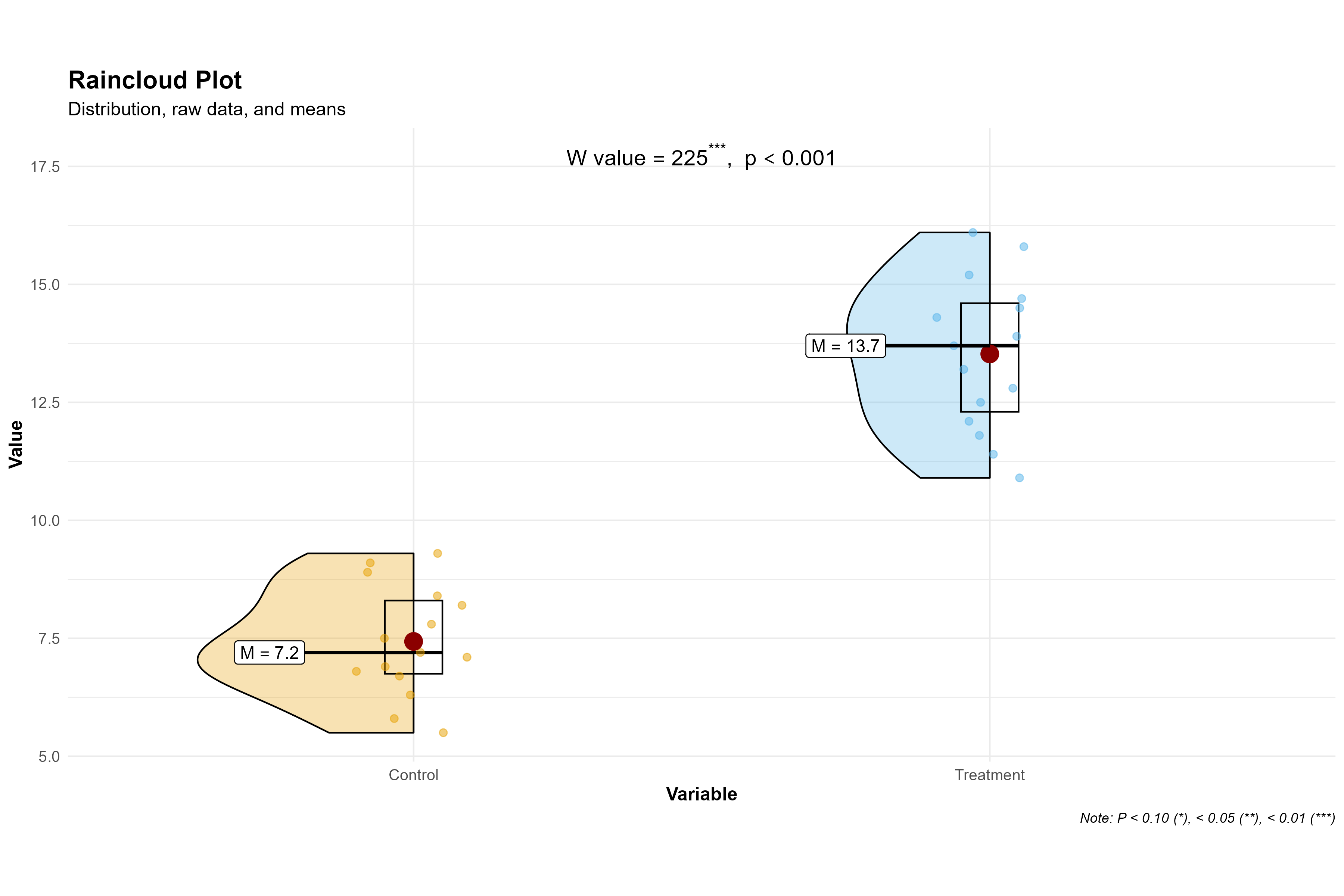
Raincloud plot. A half-violin, a box and the individual points together. Shows the distribution, the summary and the raw data in one figure, which makes it the most informative single view.
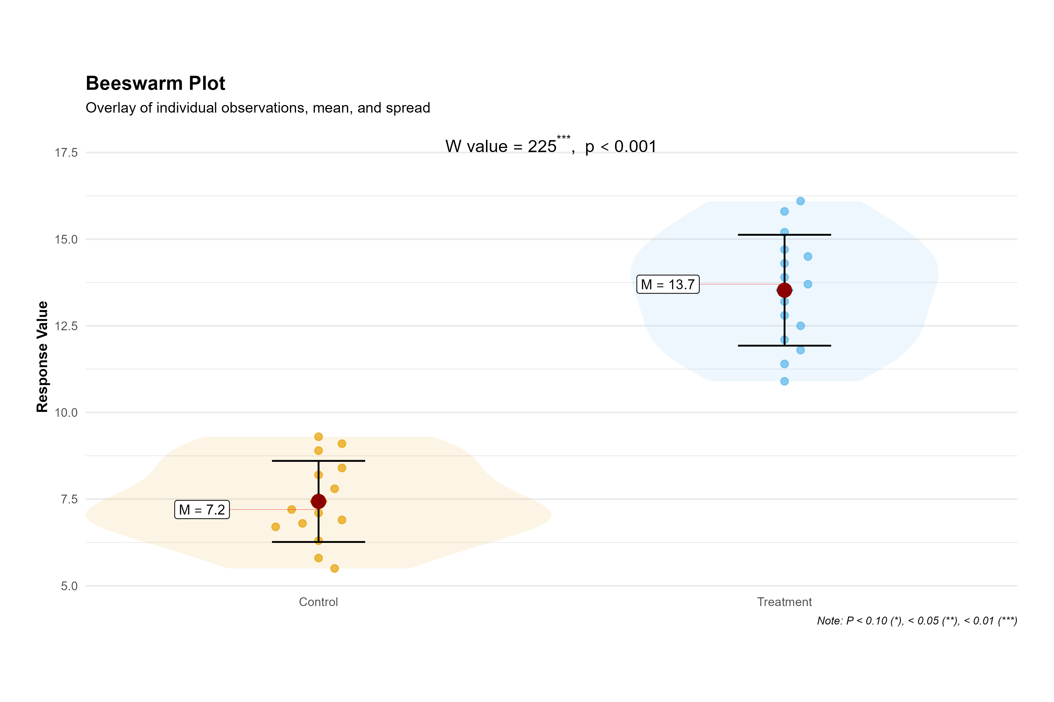
Beeswarm plot. Every observation as a point, offset sideways so none overlap. Best for small samples, where you want the reader to see the actual data rather than a summary of it.
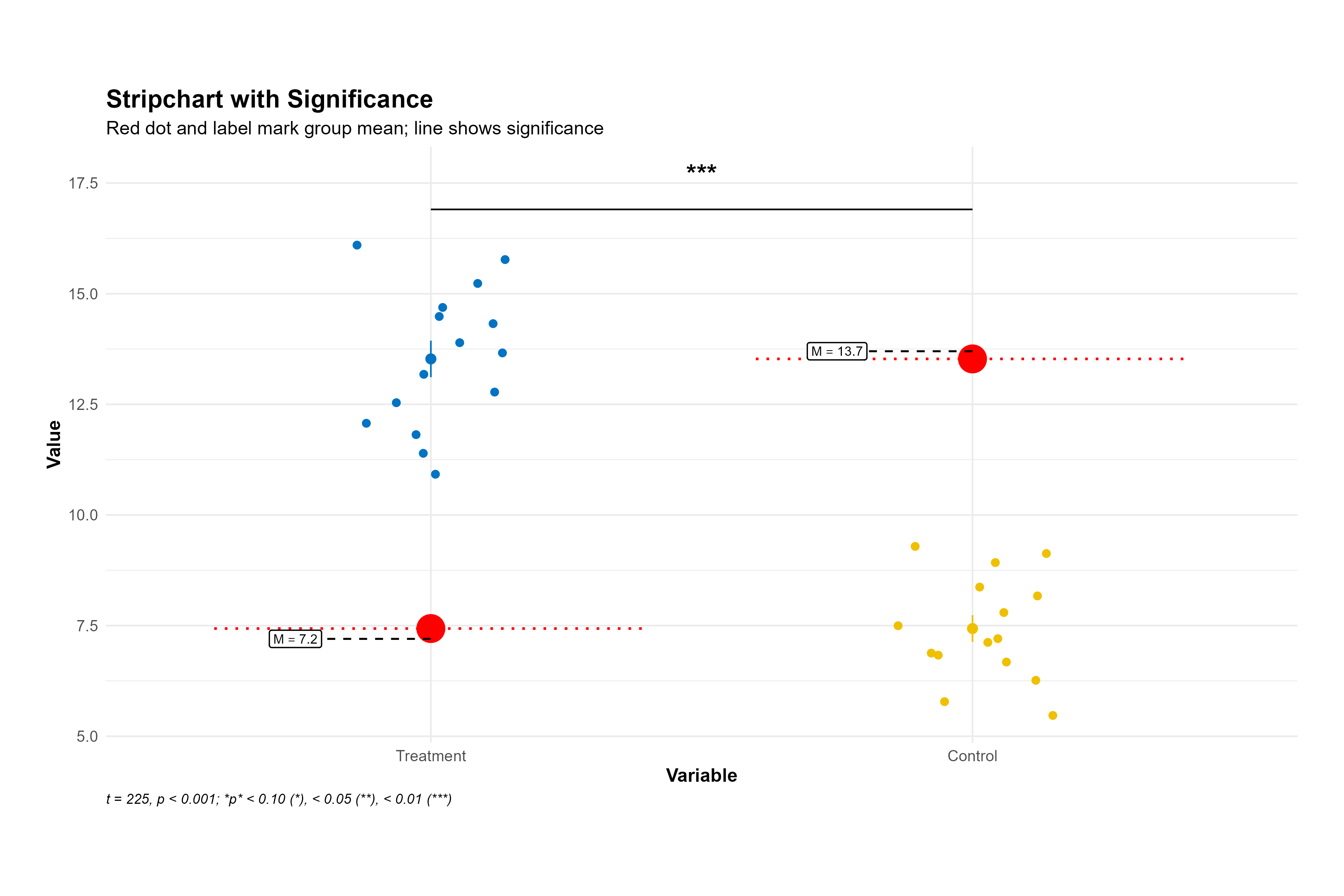
Stripchart. A simpler one-dimensional scatter of the same observations, without the beeswarm offsetting. Useful when the groups are small and the points barely overlap.
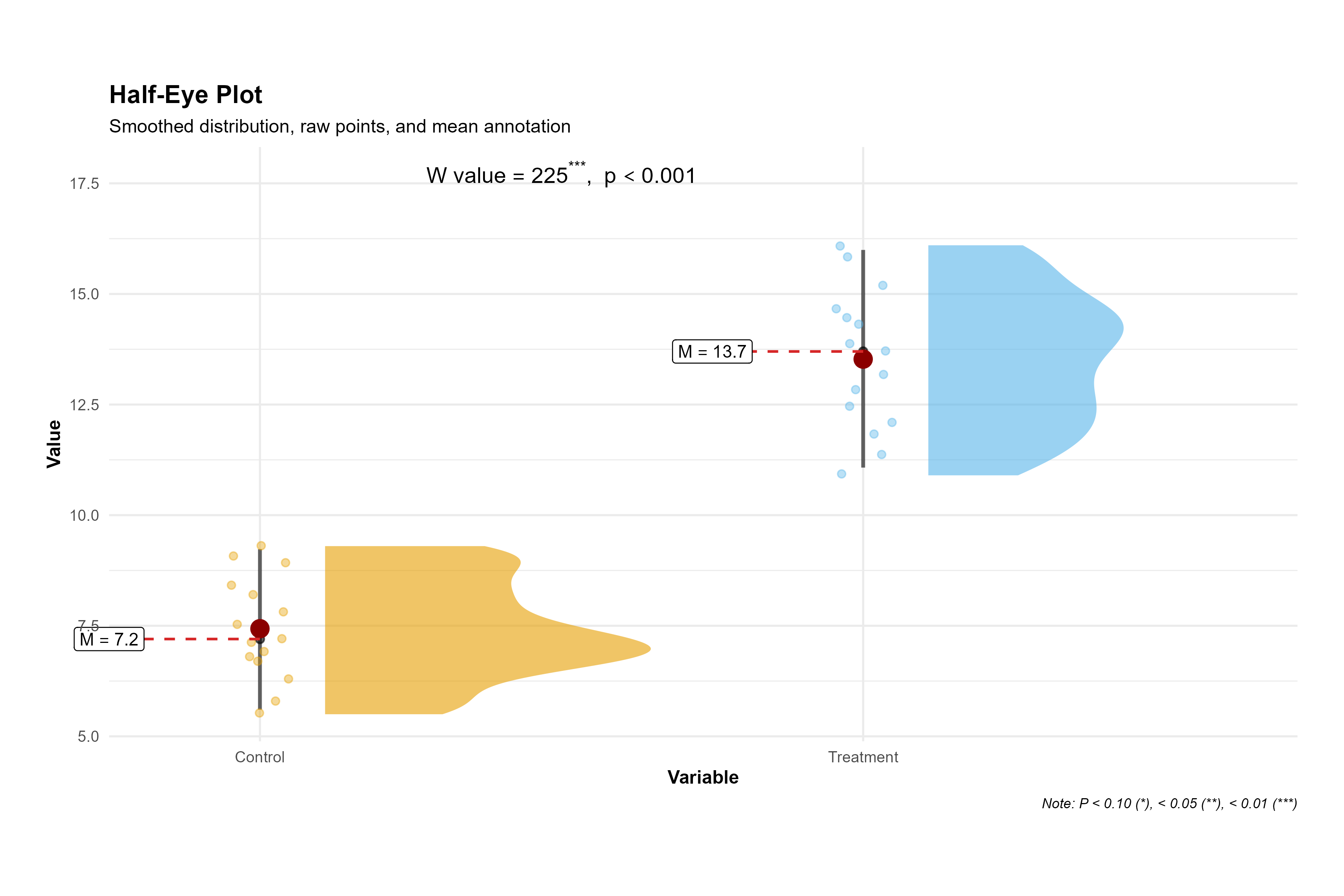
Distribution (Half-Eye) plot. The estimated density of each group with interval bars beneath it. Shows skew and multiple peaks that a box plot would hide.
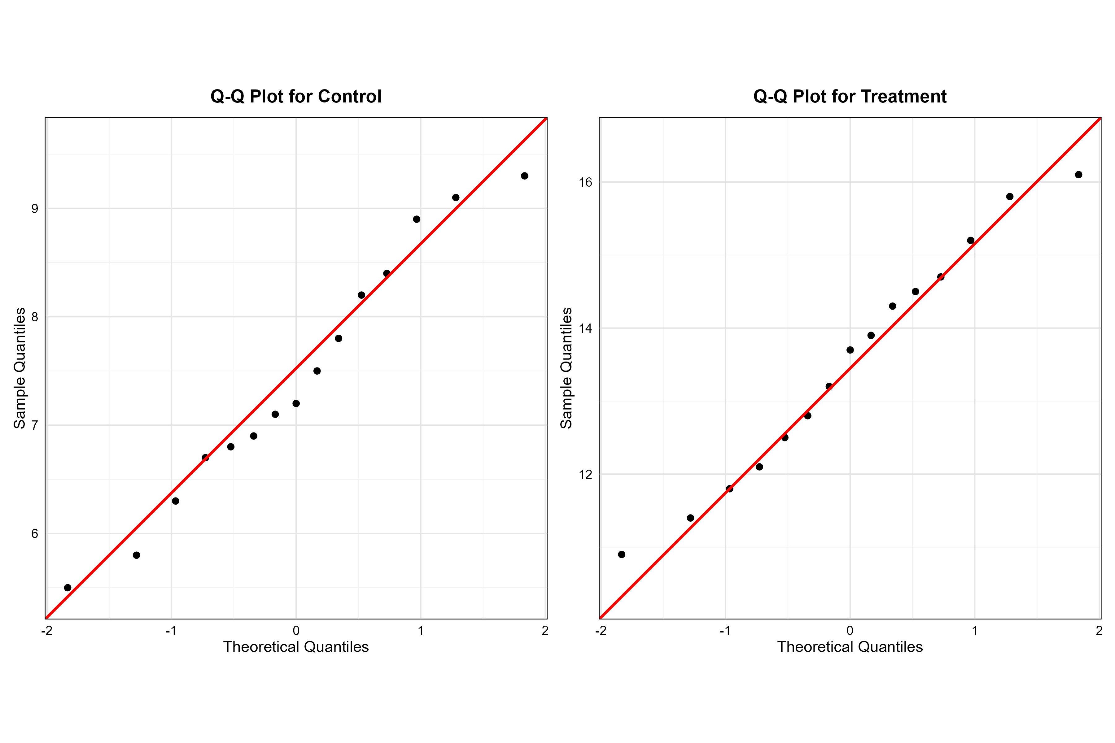
Q-Q plot. One panel per group, comparing that group’s values against a normal reference. For inspection only - neither test requires normality.
The Q-Q plot is included for inspection, not as a gatekeeper. Neither the Mann-Whitney U nor the Wilcoxon Signed-Rank test requires normality, so a curved Q-Q plot is not a reason to abandon the analysis, it is part of the reason you chose a rank-based test in the first place. Use it to understand the shape of your data and to justify that choice in your methods section.
10 Interpretation
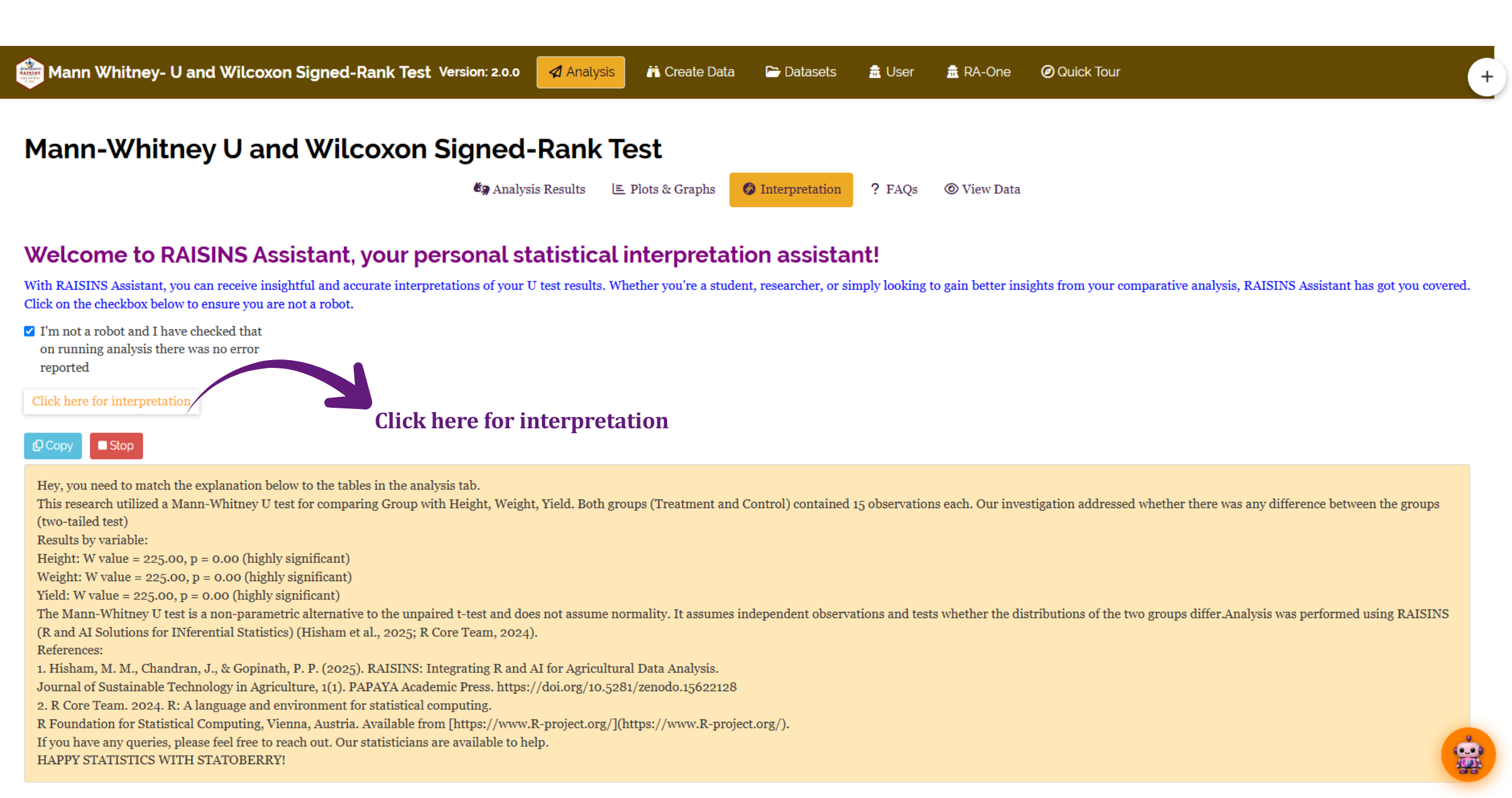
The Interpretation tab produces an automatic, plain-language write-up of the results (Figure 16): which test was run, the statistic and p-value, whether the difference was significant at your chosen α, and what that means for the two groups, phrased as prose you can adapt for a report. Unlike RA-One (Section 11), this tab does not answer follow-up questions; it produces one fixed block of text per run.
11 RA-One Chat Assistant
RA-One is the built-in chat assistant. You can open it from its navigation tab or from the floating chat bubble, visible once you are logged in.
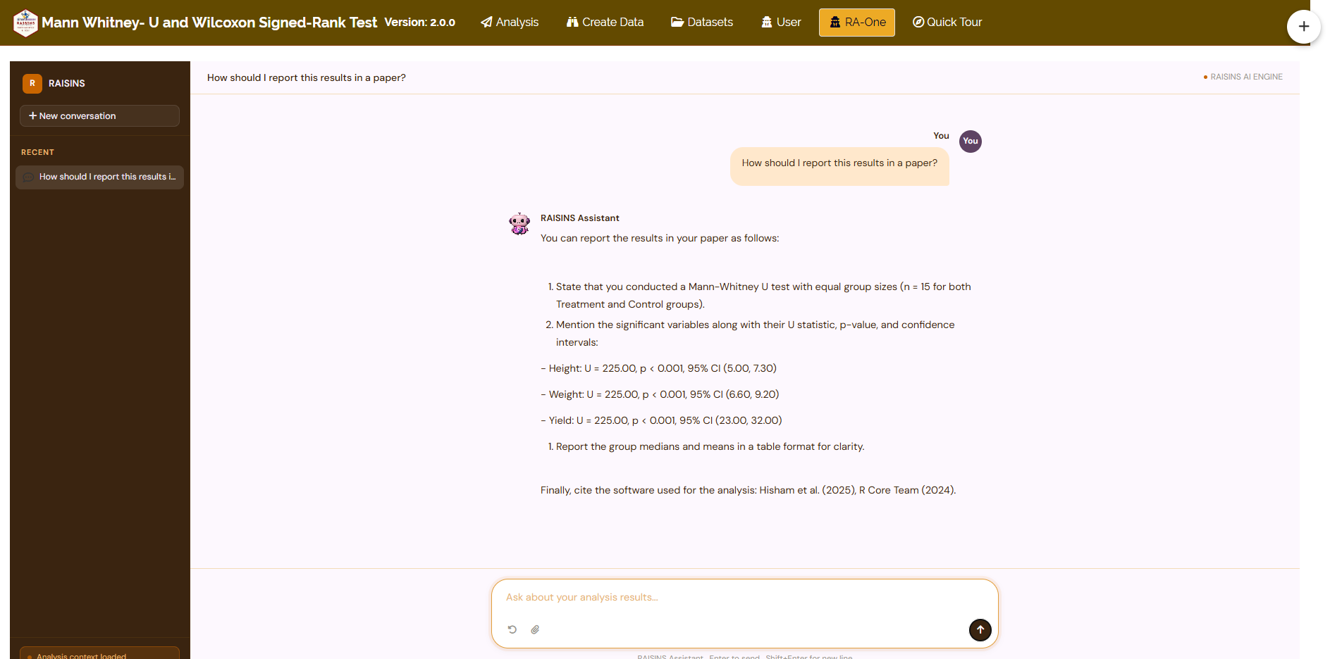
Ask questions in plain language, and RA-One answers using your own analysis results. It does not give generic advice, and it does not invent values. If a value is not available, it says so. All replies are in plain English, with no code.
It can also do more than answer questions: it will build a correctly structured data template for you (Section 6), list and hand over the bundled model datasets, advise on how many observations per group you are likely to need, and generate its own plots and result tables inside the chat.
12 Downloadable Report
Below the results table, a Download Report control exports the complete set of results as a single document, in HTML, PDF, or Word format.
The report reproduces the same per-variable table, statistics, p-values and confidence intervals shown on screen for every selected response variable, so it can be attached directly to a manuscript or shared with a supervisor without copying each table by hand. The individual plots are downloaded separately from their own tabs (Section 9), which lets you choose the format and resolution each figure needs.
13 FAQs
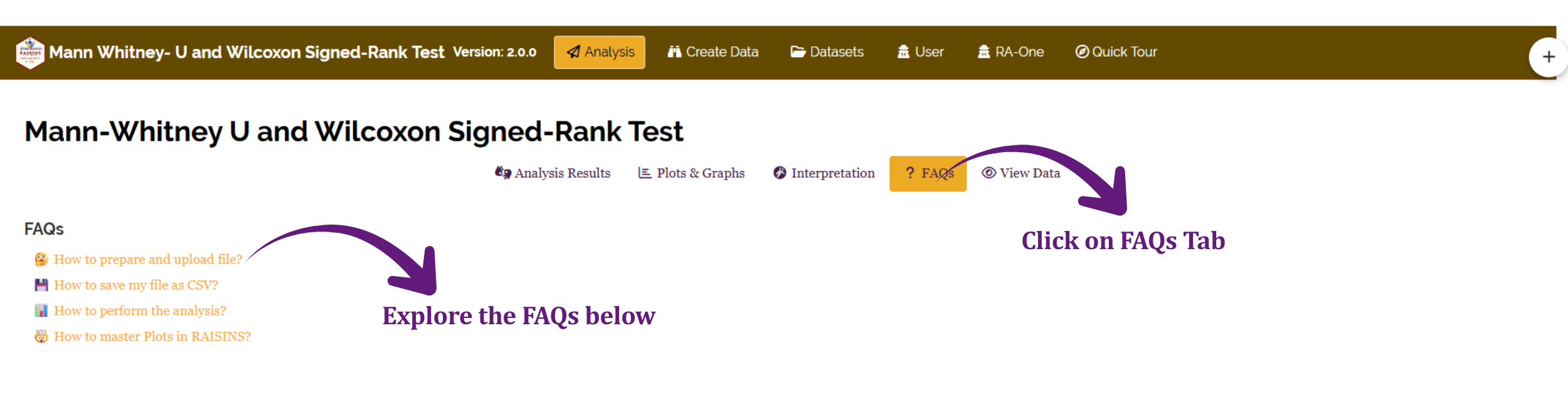
The FAQs tab collects the module’s help pages in one place: how to prepare and upload a file, how to save an Excel file as CSV, how to perform the analysis step by step, and how to get the most out of the plots. Each opens in a window without leaving the app.
If you are unsure how a feature works, start here.
14 View Data
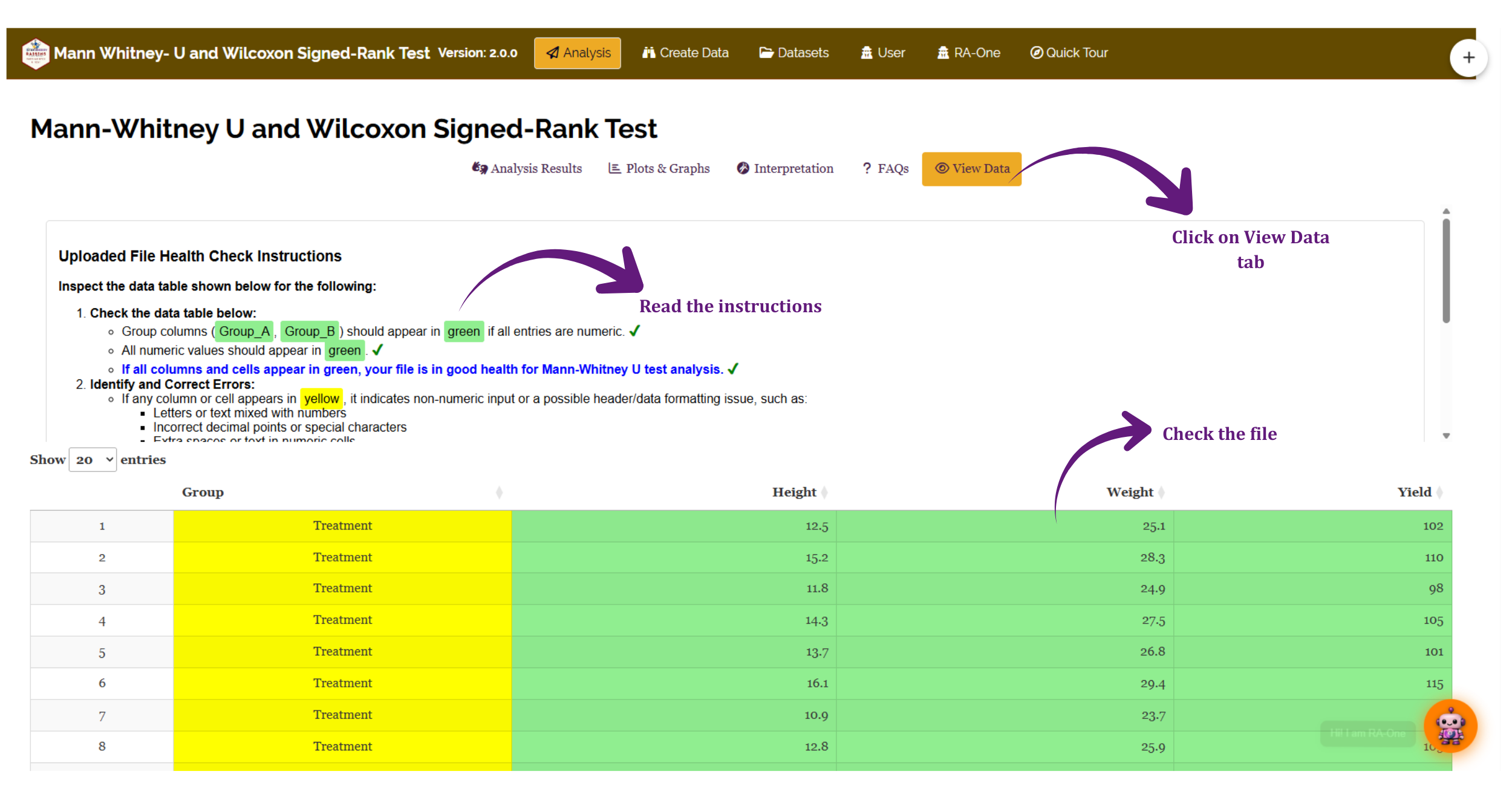
The View Data tab helps you confirm that your dataset is suitable for analysis.
When you upload a file, RAISINS runs an automated Health Check. It examines the column types and formatting, and flags any column that contains non-numeric values where a response variable is expected, missing entries, or inconsistent formatting. Group columns appear highlighted, numeric values in green, and missing values in red.
Resolve any issues reported here before selecting your Group column and response variables, so that your results are based on clean and correctly formatted data.
15 Summary
The Mann-Whitney U test answers a single question: does a numeric response tend to take larger values in one of two independent groups than in the other, without requiring that response to be normally distributed? The Wilcoxon Signed-Rank test answers the same question for measurements that come in matched pairs.
Everything else in the output exists to make that answer complete and honest: the median and IQR to describe each group in terms robust to outliers, the confidence interval to say how large the difference plausibly is rather than merely that one exists, and six plot types to show the reader the data behind the p-value. RAISINS performs all of these calculations automatically, alongside an automatic written interpretation and a downloadable report, so you can concentrate on interpreting what the results mean for your research rather than on the mechanics of computing them.
If you need help at any stage, RA-One is available at all times. You can also write to us at support@statoberry.com.
16 Appendix: A Short History of the Test
The story begins with Frank Wilcoxon, a chemist working at the Boyce Thompson Institute, whose 1945 paper “Individual Comparisons by Ranking Methods” ran to barely three pages in Biometrics Bulletin. In it he proposed both of the tests this module performs: a rank-sum procedure for two independent samples and a signed-rank procedure for paired ones. His motivation was practical rather than theoretical, he wanted a quick way to compare experimental results without the arithmetic a t-test demanded.
Two years later Henry Mann and his student Donald Whitney published “On a Test of Whether one of Two Random Variables is Stochastically Larger than the Other” in the Annals of Mathematical Statistics, developing the independent-samples case more fully, tabulating its distribution for small samples, and establishing its properties formally. Their treatment was what carried the test into general use, which is why the two-sample version is most often called the Mann-Whitney U test today, while the paired version keeps Wilcoxon’s name. The two are the same procedure, and R reports its statistic as W in acknowledgement of the earlier paper.
A third contribution completed the picture. Joseph Hodges and Erich Lehmann’s 1963 paper “Estimates of Location Based on Rank Tests” showed how to derive not just a p-value from these rank procedures but an estimate of the difference between the groups, together with a confidence interval, and to do so without assuming any particular distribution. That result is what allows a rank-based analysis to report an effect size rather than only a verdict, and it is the interval RAISINS reports alongside every test.
Today these tests are standard wherever two groups must be compared but a t-test’s assumptions cannot be relied upon, ordinal survey and sensory data, small agricultural and ecological samples, and any dataset with visible skew or outliers among them.
